
On this article, you’ll discover ways to select an applicable time sequence forecasting mannequin utilizing a transparent, four-quadrant choice matrix grounded in information complexity and enter dimensionality.
Matters we’ll cowl embody:
- The distinction between univariate and multivariate time sequence and why it issues.
- Which classical and fashionable fashions match greatest for low vs. excessive complexity information.
- Commerce-offs amongst interpretability, scalability, and accuracy throughout mannequin households.
Let’s not waste any extra time.
A Choice Matrix for Time Collection Forecasting Fashions
Picture by Editor
Introduction
Time sequence information have the added complexity of temporal dependencies, seasonality, and potential non-stationarity.
Arguably, essentially the most frequent predictive downside to handle with time sequence information is forecasting i.e. predicting future values of a variable like temperature or inventory worth based mostly on historic observations as much as the current. With so many alternative fashions for time sequence forecasting, practitioners would possibly typically discover it troublesome to decide on essentially the most appropriate method.
This text is designed to assist, by way of using a choice matrix accompanied by explanations on when and why to worker completely different fashions relying on information traits and downside sort.
The Choice Matrix
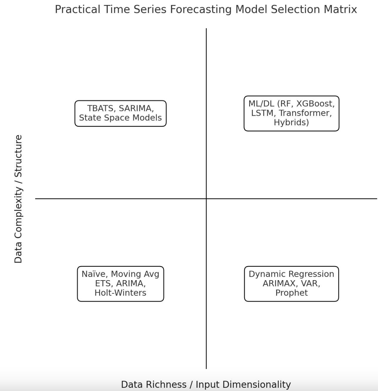
First up, we introduce the visible matrix that categorizes a set of generally used time sequence forecasting fashions relying on two main standards or dimensions.
A Choice Matrix for Time Collection Forecasting Fashions
Picture by Writer
Knowledge complexity and construction refers back to the total complexity of the time sequence dataset getting used, by way of points just like the presence or absence of stationarity patterns, seasonality, restricted vs. important noise within the information, nonlinearities, and so forth.
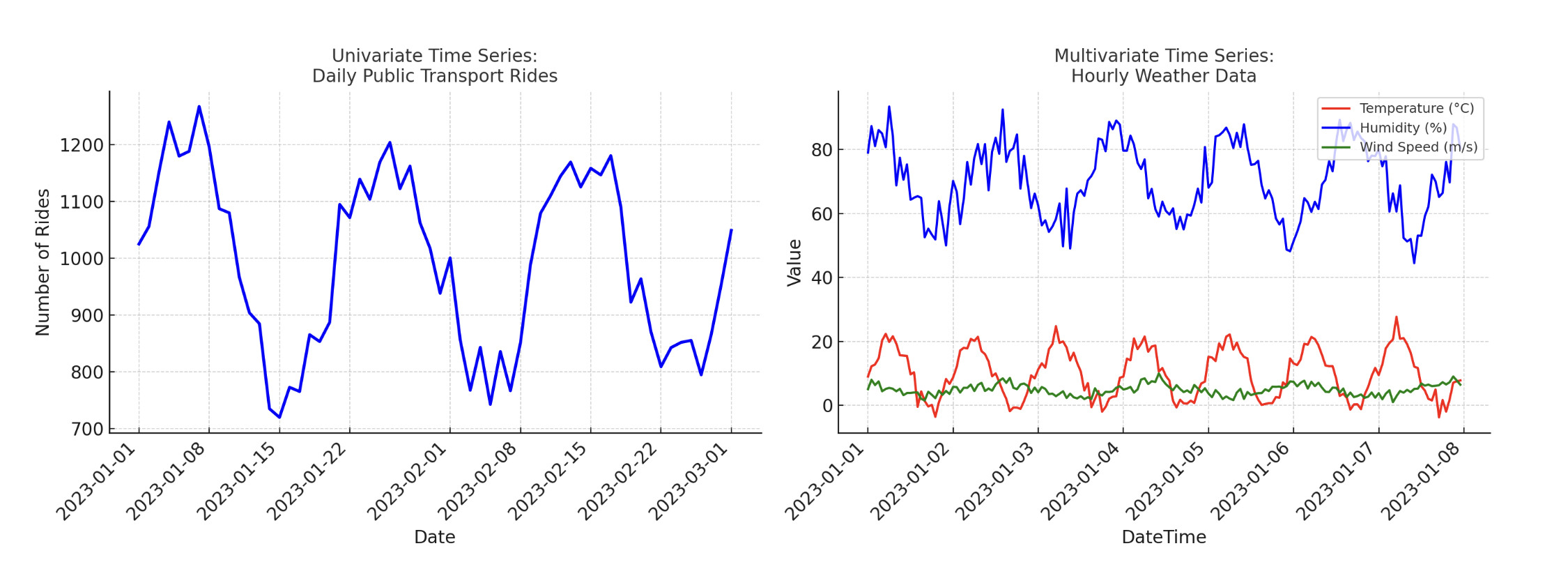
Enter dimensionality refers to the truth that, based mostly on enter information dimensionality, the time sequence may be univariate or multivariate i.e. with or without exogenous enter attributes, respectively. As an illustration, a dataset describing every day rides in a public transport system could be an instance of a univariate time sequence, whereas every day or hourly climate recordings together with wind velocity, temperature, and humidity are an instance of a multivariate time sequence.
Univariate vs Multivariate Time Collection
Picture by Writer
These two classification standards lead us to a taxonomy of time sequence forecasting fashions aligned with the matrix displayed above.
Let’s now look into every of the 4 quadrants in additional element.
1. Low-Complexity, Univariate Time Collection (Backside Left)
This quadrant encompasses forecasting issues the place the historic time sequence has low complexity — as an illustration, as a result of it’s somewhat brief, it has secure demand (pretty fixed over time), or it reveals easy developments, patterns, or seasonal construction. Usually, these sorts of time sequence additionally show approximate stationarity.
Appropriate and easy fashions which can be usually sufficient for these issues embody Naïve (for very simplistic time sequence information), or barely extra elaborate algorithms or strategies like shifting averages and their variants (easy shifting common, weighted shifting common), the basic among the many classics autoregressive built-in shifting common (ARIMA), and Holt–Winters. These are all strong fashions for easy time sequence datasets, whereas conserving interpretability and effectivity in forecasts. In the meantime, resulting from their simplicity in comparison with different superior approaches, their adaptability to points corresponding to structural breaks or exterior elements could be very restricted.
2. Low-Complexity, Multivariate Time Collection (Backside Proper)
When the time sequence nonetheless has easy patterns however is multivariate — or it’s influenced by a number of exterior elements or regression predictors — it’s higher to resort to intermediate-complexity fashions like Dynamic Regression, ARIMA with exogenous variables (ARIMAX), vector autoregression (VAR), or Prophet. These forecasting fashions can straight incorporate recognized drivers — corresponding to promotions or pricing results in buyer historic conduct information — into the forecasting, thereby performing as a hybrid between purely time-based forecasting and regression fashions.
These approaches are usually straightforward to interpret and implement, producing dependable predictions when the underlying dynamics of the dataset stay comparatively simple. Then again, regardless of having the ability to incorporate exterior variables, they nonetheless assume comparatively easy patterns and relationships and should battle with nonlinearities or hard-to-understand interactions amongst variables.
3. Excessive-Complexity, Univariate Time Collection (High Left)
Univariate time sequence exhibiting advanced patterns — like irregular developments or a number of seasonal cycles — require utilizing specialised fashions like TBATS (Trigonometric, Field–Cox transformation, ARMA errors, Development, and Seasonal parts), seasonal ARIMA (SARIMA), or state-space strategies corresponding to Kalman filter–based mostly approaches. Points like non-stationarity i.e. evolving statistical properties of the info over time, and complicated seasonal behaviors may be captured by these fashions, which makes them appropriate for forecasting in eventualities with long-term or irregular sequence with considerably “unpredictable” dynamics.
Though they outperform different fashions in dealing with inner complexities, these strategies are extra computationally intensive, and in observe, they typically require cautious fine-tuning to be exact and generalizable.
4. Excessive-Complexity, Multivariate Time Collection (High Proper)
Final of the 4 eventualities, now we have contexts with massive time sequence that comprise a number of time and/or exterior variables and current advanced or nonlinear dependencies. These difficult eventualities require superior strategies from the machine studying and deep studying panorama — for instance, ensemble strategies like Random Forests and XGBoost, recurrent neural networks corresponding to lengthy short-term reminiscence (LSTM) networks, and even deep studying architectures like transformers. Nonetheless, utilizing hybrid approaches is commonly a sensible selection in these contexts.
These data-intensive fashions are superior at capturing advanced interactions amongst variables and are scalable to very massive datasets. However on the unfavorable facet of issues, their necessities are extra demanding they usually have decrease interpretability, together with some danger of overfitting if not sufficient high-quality information is supplied to coach them.
Wrapping Up
This text took a tour of time sequence forecasting fashions and strategies from the angle of sensible selection. Primarily based on a four-quadrant choice matrix, we outlined the popular strategies to make use of in 4 various kinds of forecasting eventualities, highlighting when to make use of every group of fashions and outlining the professionals and cons of every.