
On this article, you’ll learn to cluster a group of textual content paperwork utilizing giant language mannequin embeddings and customary clustering algorithms in scikit-learn.
Subjects we’ll cowl embody:
- Why LLM-based embeddings are effectively fitted to doc clustering.
- Find out how to generate embeddings from uncooked textual content utilizing a pre-trained sentence transformer.
- Find out how to apply and examine k-means and DBSCAN for clustering embedded paperwork.
Let’s get straight to the purpose.
Doc Clustering with LLM Embeddings in Scikit-learn (click on to enlarge)
Picture by Editor
Introduction
Think about that you simply out of the blue get hold of a big assortment of unclassified paperwork and are tasked with grouping them by matter. There are conventional clustering strategies for textual content, based mostly on TF-IDF and Word2Vec, that may tackle this drawback, however they undergo from vital limitations:
- TF-IDF solely counts phrases in a textual content and depends on similarity based mostly on phrase frequencies, ignoring the underlying that means. A sentence like “the tree is huge” has an an identical illustration whether or not it refers to a pure tree or a choice tree classifier utilized in machine studying.
- Word2Vec captures relationships between particular person phrases to kind embeddings (numerical vector representations), nevertheless it doesn’t explicitly mannequin full context throughout longer textual content sequences.
In the meantime, fashionable embeddings generated by giant language fashions, akin to sentence transformer fashions, are generally superior. They seize contextual semantics — for instance, distinguishing pure timber from resolution timber — and encode total, document-level that means. Furthermore, these embeddings are produced by fashions pre-trained on thousands and thousands of texts, that means they already comprise a considerable quantity of basic language information.
This text follows up on a earlier tutorial, the place we discovered find out how to convert uncooked textual content into giant language mannequin embeddings that can be utilized as options for downstream machine studying duties. Right here, we focus particularly on utilizing embeddings from a group of paperwork for clustering based mostly on similarity, with the purpose of figuring out widespread matters amongst paperwork in the identical cluster.
Step-by-Step Information
Let’s stroll by the complete course of utilizing Python.
Relying in your improvement surroundings or pocket book configuration, it’s possible you’ll must pip set up among the libraries imported under. Assuming they’re already accessible, we begin by importing the required modules and lessons, together with KMeans, scikit-learn’s implementation of the k-means clustering algorithm:
|
import pandas as pd import numpy as np from sentence_transformers import SentenceTransformer from sklearn.cluster import KMeans from sklearn.decomposition import PCA from sklearn.metrics import silhouette_score, adjusted_rand_score from sklearn.preprocessing import LabelEncoder import matplotlib.pyplot as plt import seaborn as sns
# Configurations for clearer visualizations sns.set_style(“whitegrid”) plt.rcParams[‘figure.figsize’] = (12, 6) |
Subsequent, we load the dataset. We’ll use a BBC Information dataset containing articles labeled by matter, with a public model accessible from a Google-hosted dataset repository:
|
url = “https://storage.googleapis.com/dataset-uploader/bbc/bbc-text.csv” df = pd.read_csv(url)
print(f“Dataset loaded: {len(df)} paperwork”) print(f“Classes: {df[‘category’].distinctive()}n”) print(df[‘category’].value_counts()) |
Right here, we solely show details about the classes to get a way of the ground-truth matters assigned to every doc. The dataset comprises 2,225 paperwork within the model used on the time of writing.
At this level, we’re prepared for the 2 primary steps of the workflow: producing embeddings from uncooked textual content and clustering these embeddings.
Producing Embeddings with a Pre-Skilled Mannequin
Libraries akin to sentence_transformers make it simple to make use of a pre-trained mannequin for duties like producing embeddings from textual content. The workflow consists of loading an acceptable mannequin — akin to all-MiniLM-L6-v2, a light-weight mannequin educated to provide 384-dimensional embeddings — and operating inference over the dataset to transform every doc right into a numerical vector that captures its total semantics.
We begin by loading the mannequin:
|
# Load embeddings mannequin (downloaded mechanically on first use) print(“Loading embeddings mannequin…”) mannequin = SentenceTransformer(‘all-MiniLM-L6-v2’)
# This mannequin converts textual content right into a 384-dimensional vector print(f“Mannequin loaded. Embedding dimension: {mannequin.get_sentence_embedding_dimension()}”) |
Subsequent, we generate embeddings for all paperwork:
|
# Convert all paperwork into embedding vectors print(“Producing embeddings (this will likely take a couple of minutes)…”)
texts = df[‘text’].tolist() embeddings = mannequin.encode( texts, show_progress_bar=True, batch_size=32 # Batch processing for effectivity )
print(f“Embeddings generated: matrix measurement is {embeddings.form}”) print(f” → Every doc is now represented by {embeddings.form[1]} numeric values”) |
Recall that an embedding is a high-dimensional numerical vector. Paperwork which might be semantically related are anticipated to have embeddings which might be shut to one another on this vector area.
Clustering Doc Embeddings with Ok-Means
Making use of the k-means clustering algorithm with scikit-learn is easy. We cross within the embedding matrix and specify the variety of clusters to search out. Whereas this quantity should be chosen prematurely for k-means, we will leverage prior information of the dataset’s ground-truth classes on this instance. In different settings, methods such because the elbow technique may also help information this alternative.
The next code applies k-means and evaluates the outcomes utilizing a number of metrics, together with the Adjusted Rand Index (ARI). ARI is a permutation-invariant metric that compares the cluster assignments with the true class labels. Values nearer to 1 point out stronger settlement with the bottom fact.
|
n_clusters = 5
kmeans = KMeans(n_clusters=n_clusters, random_state=42, n_init=10) kmeans_labels = kmeans.fit_predict(embeddings)
# Analysis towards ground-truth classes le = LabelEncoder() true_labels = le.fit_transform(df[‘category’])
print(” Ok-Means Outcomes:”) print(f” Silhouette Rating: {silhouette_score(embeddings, kmeans_labels):.3f}”) print(f” Adjusted Rand Index: {adjusted_rand_score(true_labels, kmeans_labels):.3f}”) print(f” Distribution: {pd.Sequence(kmeans_labels).value_counts().sort_index().tolist()}”) |
Instance output:
|
Ok–Means Outcomes: Silhouette Rating: 0.066 Adjusted Rand Index: 0.899 Distribution: [376, 414, 517, 497, 421] |
Clustering Doc Embeddings with DBSCAN
In its place, we will apply DBSCAN, a density-based clustering algorithm that mechanically infers the variety of clusters based mostly on level density. As a substitute of specifying the variety of clusters, DBSCAN requires parameters akin to eps (the neighborhood radius) and min_samples:
|
from sklearn.cluster import DBSCAN
# DBSCAN usually works higher with cosine distance for textual content embeddings dbscan = DBSCAN(eps=0.5, min_samples=5, metric=‘cosine’) dbscan_labels = dbscan.fit_predict(embeddings)
# Depend clusters (-1 signifies noise factors) n_clusters_found = len(set(dbscan_labels)) – (1 if –1 in dbscan_labels else 0) n_noise = record(dbscan_labels).rely(–1)
print(“nDBSCAN Outcomes:”) print(f” Clusters discovered: {n_clusters_found}”) print(f” Noise paperwork: {n_noise}”) print(f” Silhouette Rating: {silhouette_score(embeddings[dbscan_labels != -1], dbscan_labels[dbscan_labels != -1]):.3f}”) print(f” Adjusted Rand Index: {adjusted_rand_score(true_labels, dbscan_labels):.3f}”) print(f” Distribution: {pd.Sequence(dbscan_labels).value_counts().sort_index().to_dict()}”) |
DBSCAN is very delicate to its hyperparameters, so reaching good outcomes usually requires cautious tuning utilizing systematic search methods.
As soon as affordable parameters have been recognized, it may be informative to visually examine the clustering outcomes. The next code initiatives the embeddings into two dimensions utilizing principal element evaluation (PCA) and plots the true classes alongside the k-means and DBSCAN cluster assignments:
|
1 2 3 4 5 6 7 8 9 10 11 12 13 14 15 16 17 18 19 20 21 22 23 24 25 26 27 28 29 30 31 32 33 34 35 36 37 38 39 40 41 42 43 44 45 46 47 48 49 50 51 52 53 |
# Scale back embeddings to 2D for visualization pca = PCA(n_components=2, random_state=42) embeddings_2d = pca.fit_transform(embeddings)
# Create comparative visualization fig, axes = plt.subplots(1, 3, figsize=(18, 5))
# Plot 1: True classes category_colors = {cat: i for i, cat in enumerate(df[‘category’].distinctive())} color_map = df[‘category’].map(category_colors)
axes[0].scatter( embeddings_2d[:, 0], embeddings_2d[:, 1], c=color_map, cmap=‘Set2’, alpha=0.6, s=30 ) axes[0].set_title(‘True Classes’, fontsize=12, fontweight=‘daring’) axes[0].set_xlabel(‘PC1’) axes[0].set_ylabel(‘PC2’)
# Plot 2: Ok-Means scatter2 = axes[1].scatter( embeddings_2d[:, 0], embeddings_2d[:, 1], c=kmeans_labels, cmap=‘viridis’, alpha=0.6, s=30 ) axes[1].set_title(f‘Ok-Means (ok={n_clusters})’, fontsize=12, fontweight=‘daring’) axes[1].set_xlabel(‘PC1’) axes[1].set_ylabel(‘PC2’) plt.colorbar(scatter2, ax=axes[1])
# Plot 3: DBSCAN scatter3 = axes[2].scatter( embeddings_2d[:, 0], embeddings_2d[:, 1], c=dbscan_labels, cmap=‘plasma’, alpha=0.6, s=30 ) axes[2].set_title(f‘DBSCAN ({n_clusters_found} clusters + noise)’, fontsize=12, fontweight=‘daring’) axes[2].set_xlabel(‘PC1’) axes[2].set_ylabel(‘PC2’) plt.colorbar(scatter3, ax=axes[2])
plt.tight_layout() plt.present() |
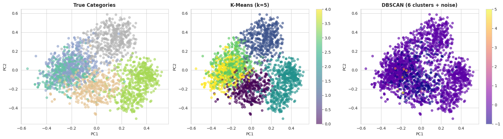
With the default DBSCAN settings, k-means sometimes performs significantly better on this dataset. There are two primary causes for this:
- DBSCAN suffers from the curse of dimensionality, and 384-dimensional embeddings may be difficult for density-based strategies.
- Ok-means performs effectively when clusters are comparatively effectively separated, which is the case for the BBC Information dataset because of the clear topical construction of the paperwork.
Wrapping Up
On this article, we demonstrated find out how to cluster a group of textual content paperwork utilizing embedding representations generated by pre-trained giant language fashions. After remodeling uncooked textual content into numerical vectors, we utilized conventional clustering methods — k-means and DBSCAN — to group semantically related paperwork and consider their efficiency towards identified matter labels.