
The success of machine studying pipelines will depend on characteristic engineering as their important basis. The 2 strongest strategies for dealing with time collection information are lag options and rolling options, in line with your superior methods. The flexibility to make use of these methods will improve your mannequin efficiency for gross sales forecasting, inventory worth prediction, and demand planning duties.
This information explains lag and rolling options by exhibiting their significance and offering Python implementation strategies and potential implementation challenges by means of working code examples.
What’s Characteristic Engineering in Time Collection?
Time collection characteristic engineering creates new enter variables by means of the method of reworking uncooked temporal information into options that allow machine studying fashions to detect temporal patterns extra successfully. Time collection information differs from static datasets as a result of it maintains a sequential construction, which requires observers to grasp that previous observations affect what’s going to come subsequent.
The standard machine studying fashions XGBoost, LightGBM, and Random Forests lack built-in capabilities to course of time. The system requires particular indicators that want to indicate previous occasions that occurred earlier than. The implementation of lag options along with rolling options serves this objective.
What Are Lag Options?
A lag characteristic is just a previous worth of a variable that has been shifted ahead in time till it matches the present information level. The gross sales prediction for right now will depend on three completely different gross sales info sources, which embody yesterday’s gross sales information and each seven-day and thirty-day gross sales information.
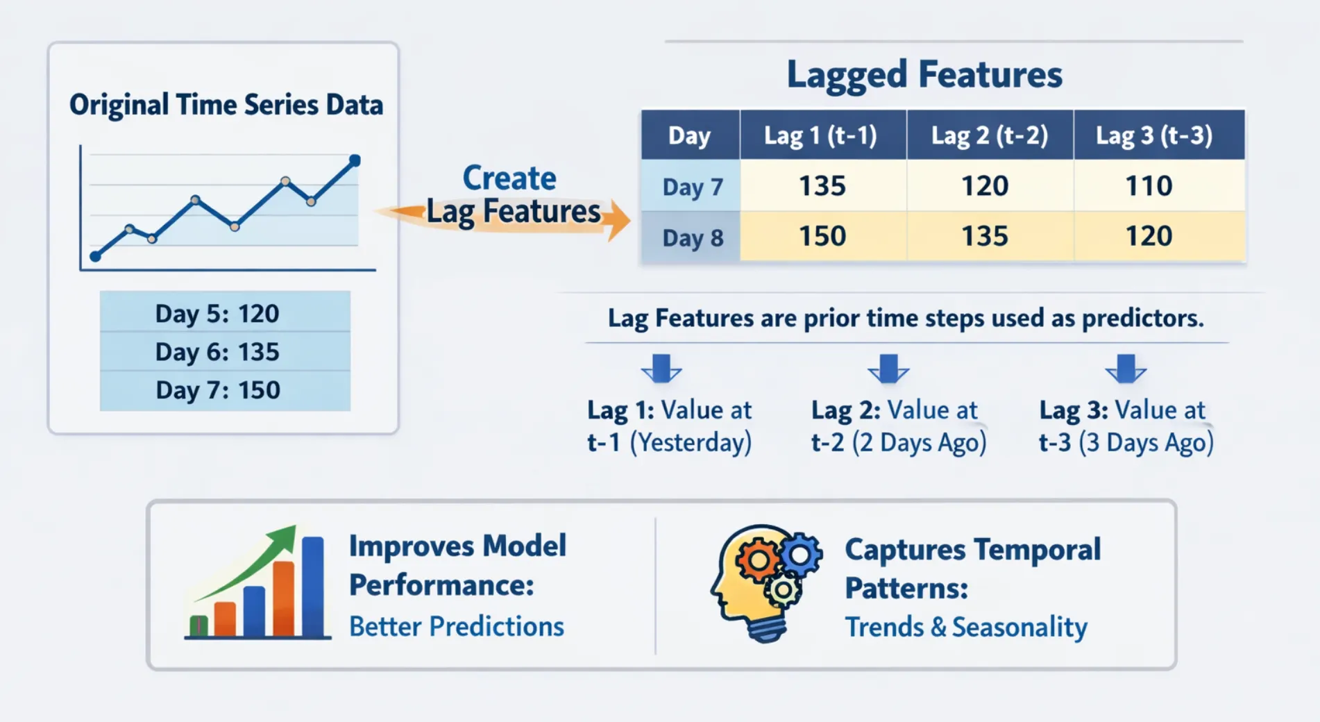
Why Lag Options Matter
- They symbolize the connection between completely different time intervals when a variable reveals its previous values.
- The strategy permits seasonal and cyclical patterns to be encoded while not having difficult transformations.
- The strategy offers easy computation along with clear outcomes.
- The system works with all machine studying fashions that use tree constructions and linear strategies.
Implementing LAG Options in Python
import pandas as pd
import numpy as np
# Create a pattern time collection dataset
np.random.seed(42)
dates = pd.date_range(begin="2024-01-01", intervals=15, freq='D')
gross sales = [200, 215, 198, 230, 245, 210, 225, 260, 275, 240, 255, 290, 305, 270, 285]
df = pd.DataFrame({'date': dates, 'gross sales': gross sales})
df.set_index('date', inplace=True)
# Create lag options
df['lag_1'] = df['sales'].shift(1)
df['lag_3'] = df['sales'].shift(3)
df['lag_7'] = df['sales'].shift(7)
print(df.head(12))
Output:
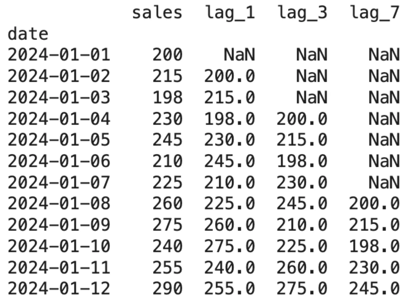
The preliminary look of NaN values demonstrates a type of information loss that happens due to lagging. This issue turns into essential for figuring out the variety of lags to be created.
Selecting the Proper Lag Values
The choice course of for optimum lags calls for scientific strategies that get rid of random choice as an possibility. The next strategies have proven profitable leads to apply:
- The information of the area helps loads, like Weekly gross sales information? Add lags at 7, 14, 28 days. Hourly vitality information? Strive 24 to 48 hours.
- Autocorrelation Perform ACF allows customers to find out which lags present vital hyperlinks to their goal variable by means of its statistical detection technique.
- The mannequin will establish which lags maintain the best significance after you full the coaching process.
What Are Rolling (Window) Options?
The rolling options perform as window options that function by transferring by means of time to calculate variable portions. The system offers you with aggregated statistics, which embody imply, median, customary deviation, minimal, and most values for the final N intervals as an alternative of exhibiting you a single previous worth.
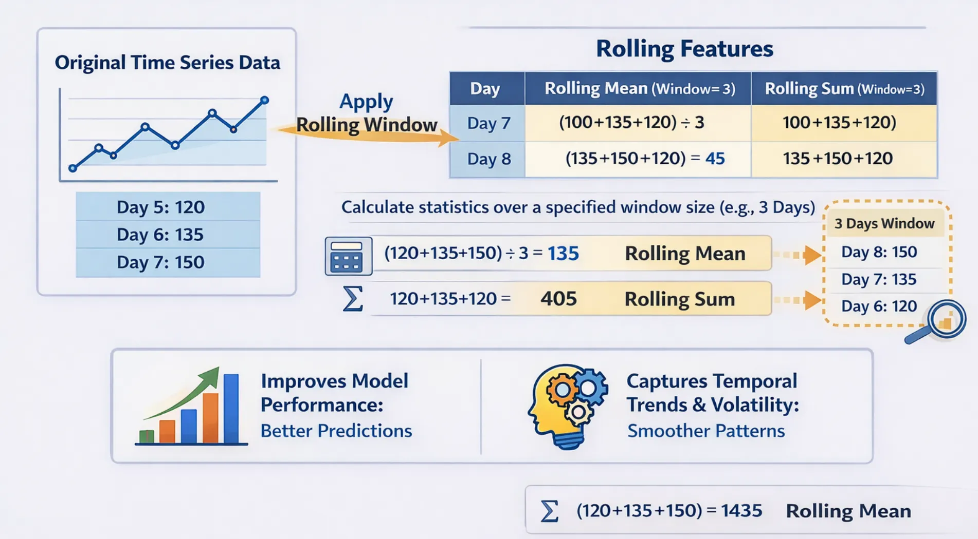
Why Rolling Options Matter?
The next options present wonderful capabilities to carry out their designated duties:
- The method eliminates noise components whereas it reveals the basic progress patterns.
- The system allows customers to watch short-term worth fluctuations that happen inside particular time intervals.
- The system allows customers to watch short-term worth fluctuations that happen inside particular time intervals.
- The system identifies uncommon behaviour when current values transfer away from the established rolling common.
The next aggregations set up their presence as customary apply in rolling home windows:
- The commonest technique of pattern smoothing makes use of a rolling imply as its main technique.
- The rolling customary deviation perform calculates the diploma of variability that exists inside a specified time window.
- The rolling minimal and most features establish the best and lowest values that happen throughout an outlined time interval/interval.
- The rolling median perform offers correct outcomes for information that features outliers and reveals excessive ranges of noise.
- The rolling sum perform helps monitor complete quantity or complete rely throughout time.
Implementing Rolling Options in Python
import pandas as pd
import numpy as np
np.random.seed(42)
dates = pd.date_range(begin="2024-01-01", intervals=15, freq='D')
gross sales = [200, 215, 198, 230, 245, 210, 225, 260, 275, 240, 255, 290, 305, 270, 285]
df = pd.DataFrame({'date': dates, 'gross sales': gross sales})
df.set_index('date', inplace=True)
# Rolling options with window measurement of three and seven
df['roll_mean_3'] = df['sales'].shift(1).rolling(window=3).imply()
df['roll_std_3'] = df['sales'].shift(1).rolling(window=3).std()
df['roll_max_3'] = df['sales'].shift(1).rolling(window=3).max()
df['roll_mean_7'] = df['sales'].shift(1).rolling(window=7).imply()
print(df.spherical(2))
Output:
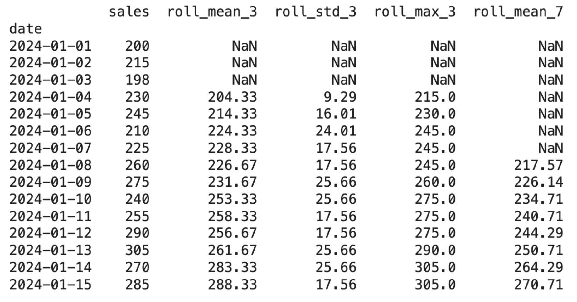
The .shift(1) perform should be executed earlier than the .rolling() perform as a result of it creates an important connection between each features. The system wants this mechanism as a result of it would create rolling calculations that rely solely on historic information with out utilizing any present information.
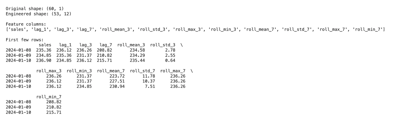
Combining Lag and Rolling Options: A Manufacturing-Prepared Instance
In precise machine studying time collection workflows, researchers create their very own hybrid characteristic set, which incorporates each lag options and rolling options. We offer you an entire characteristic engineering perform, which you should use for any mission.
import pandas as pd
import numpy as np
def create_time_features(df, target_col, lags=[1, 3, 7], home windows=[3, 7]):
"""
Create lag and rolling options for time collection ML.
Parameters:
df : DataFrame with datetime index
target_col : Identify of the goal column
lags : Checklist of lag intervals
home windows : Checklist of rolling window sizes
Returns:
DataFrame with new options
"""
df = df.copy()
# Lag options
for lag in lags:
df[f'lag_{lag}'] = df[target_col].shift(lag)
# Rolling options (shift by 1 to keep away from leakage)
for window in home windows:
shifted = df[target_col].shift(1)
df[f'roll_mean_{window}'] = shifted.rolling(window).imply()
df[f'roll_std_{window}'] = shifted.rolling(window).std()
df[f'roll_max_{window}'] = shifted.rolling(window).max()
df[f'roll_min_{window}'] = shifted.rolling(window).min()
return df.dropna() # Drop rows with NaN from lag/rolling

# Pattern utilization
np.random.seed(0)
dates = pd.date_range('2024-01-01', intervals=60, freq='D')
gross sales = 200 + np.cumsum(np.random.randn(60) * 5)
df = pd.DataFrame({'gross sales': gross sales}, index=dates)
df_features = create_time_features(df, 'gross sales', lags=[1, 3, 7], home windows=[3, 7])
print(f"Authentic form: {df.form}")
print(f"Engineered form: {df_features.form}")
print(f"nFeature columns:n{checklist(df_features.columns)}")
print(f"nFirst few rows:n{df_features.head(3).spherical(2)}")
Output:
Widespread Errors and Learn how to Keep away from Them
Probably the most extreme error in time collection characteristic engineering happens when information leakage, which reveals upcoming information to testing options, results in deceptive mannequin efficiency.
Key errors to be careful for:
- The method requires a .shift(1) command earlier than beginning the .rolling() perform. The present remark will develop into a part of the rolling window as a result of rolling requires the primary remark to be shifted.
- Knowledge loss happens by means of the addition of lags as a result of every lag creates NaN rows. The 100-row dataset will lose 30% of its information as a result of 30 lags require 30 NaN rows to be created.
- The method requires separate window measurement experiments as a result of completely different traits want completely different window sizes. The method requires testing brief home windows, which vary from 3 to five, and lengthy home windows, which vary from 14 to 30.
- The manufacturing atmosphere requires you to compute rolling and lag options from precise historic information, which you’ll use throughout inference time as an alternative of utilizing your coaching information.
When to Use Lag vs. Rolling Options
| Use Case | Advisable Options |
|---|---|
| Robust autocorrelation in information | Lag options (lag-1, lag-7) |
| Noisy sign, want smoothing | Rolling imply |
| Seasonal patterns (weekly) | Lag-7, lag-14, lag-28 |
| Pattern detection | Rolling imply over lengthy home windows |
| Anomaly detection | Deviation from rolling imply |
| Capturing variability / threat | Rolling customary deviation, rolling vary |
Conclusion
The time collection machine studying infrastructure makes use of lag options and rolling options as its important elements. The 2 strategies set up a pathway from unprocessed sequential information to the organized information format that machine studying fashions require for his or her coaching course of. The strategies develop into the best affect issue for forecasting accuracy when customers execute them with exact information dealing with and window choice strategies, and their contextual understanding of the precise subject.
The most effective half? They supply clear explanations that require minimal computing assets and performance with any machine studying mannequin. These options will profit you no matter whether or not you employ XGBoost for demand forecasting, LSTM for anomaly detection, or linear regression for baseline fashions.
Gen AI Intern at Analytics Vidhya
Division of Pc Science, Vellore Institute of Expertise, Vellore, India
I’m presently working as a Gen AI Intern at Analytics Vidhya, the place I contribute to revolutionary AI-driven options that empower companies to leverage information successfully. As a final-year Pc Science pupil at Vellore Institute of Expertise, I convey a strong basis in software program growth, information analytics, and machine studying to my function.
Be happy to attach with me at [email protected]
Login to proceed studying and luxuriate in expert-curated content material.