
Don’t know a lot about Bitcoin or its worth fluctuations however wish to make funding choices to make income? This machine studying mannequin has your again. It could predict the costs approach higher than an astrologer. On this article, we are going to construct an ML mannequin for forecasting and predicting Bitcoin worth, utilizing ZenML and MLflow. So let’s begin our journey to grasp how anybody can use ML and MLOps instruments to foretell the longer term.
Studying Targets
- Study to fetch dwell knowledge utilizing API effectively.
- Perceive what ZenML is, why we use MLflow, and how one can combine it with ZenML.
- Discover the deployment course of for machine studying fashions, from thought to manufacturing.
- Uncover the right way to create a user-friendly Streamlit app for interactive machine-learning mannequin predictions.
This text was revealed as part of the Knowledge Science Blogathon.
Drawback Assertion
Bitcoin costs are extremely risky, and making predictions is subsequent to not possible. In our mission, we’re utilizing MLOps’ finest practices to construct an LSTM mannequin to forecast Bitcoin costs and traits.
Earlier than implementing the mission let’s have a look at the mission structure.
Challenge Implementation
Let’s start by accessing the API.
Why are we doing this? You may get historic Bitcoin worth knowledge from totally different datasets, however with an API, we will have entry to dwell market knowledge.
Step 1: Accessing the API
import requests
import pandas as pd
from dotenv import load_dotenv
import os

# Load the .env file
load_dotenv()

def fetch_crypto_data(api_uri):
    response = requests.get(
        api_uri,
        params={
            "market": "cadli",
            "instrument": "BTC-USD",
            "restrict": 5000,
            "combination": 1,
            "fill": "true",
            "apply_mapping": "true",
            "response_format": "JSON"
        },
        headers={"Content material-type": "software/json; charset=UTF-8"}
    )

    if response.status_code == 200:
        print('API Connection Profitable! nFetching the info...')

        knowledge = response.json()
        data_list = knowledge.get('Knowledge', [])

        df = pd.DataFrame(data_list)

        df['DATE'] = pd.to_datetime(df['TIMESTAMP'], unit="s")

        return df  # Return the DataFrame
    else:
        increase Exception(f"API Error: {response.status_code} - {response.textual content}")
Step 2: Connecting to Database Utilizing MongoDB
MongoDB is a NoSQL database recognized for its adaptability, expandability, and skill to retailer unstructured knowledge in a JSON-like format.
import os
from pymongo import MongoClient
from dotenv import load_dotenv
from knowledge.administration.api import fetch_crypto_data  # Import the API perform
import pandas as pd

load_dotenv()

MONGO_URI = os.getenv("MONGO_URI")
API_URI = os.getenv("API_URI")

consumer = MongoClient(MONGO_URI, ssl=True, ssl_certfile=None, ssl_ca_certs=None)
db = consumer['crypto_data']
assortment = db['historical_data']

attempt:
    latest_entry = assortment.find_one(type=[("DATE", -1)])  # Discover the newest date
    if latest_entry:
        last_date = pd.to_datetime(latest_entry['DATE']).strftime('%Y-%m-%d')
    else:
        last_date="2011-03-27"  # Default begin date if MongoDB is empty

    print(f"Fetching knowledge ranging from {last_date}...")
    new_data_df = fetch_crypto_data(API_URI)

    if latest_entry:
        new_data_df = new_data_df[new_data_df['DATE'] > last_date]

    if not new_data_df.empty:
        data_to_insert = new_data_df.to_dict(orient="data")
        end result = assortment.insert_many(data_to_insert)
        print(f"Inserted {len(end result.inserted_ids)} new data into MongoDB.")
    else:
        print("No new knowledge to insert.")
besides Exception as e:
    print(f"An error occurred: {e}")
This code connects to MongoDB, retrieves Bitcoin worth knowledge by way of an API, and updates the database with all new entries after the newest logged date.
Introducing ZenML
ZenML is an open-source platform tailor-made for machine studying operations, supporting the creation of versatile and production-ready pipelines. Moreover, ZenML integrates with a number of machine studying instruments like MLflow, BentoML, and many others., to create seamless ML pipelines.
⚠️ If you’re a Home windows person, attempt to set up wsl in your system. Zenml doesn’t help Home windows.
On this mission, we are going to implement a standard pipeline, which makes use of ZenML, and we will likely be integrating MLflow with ZenML, for experiment monitoring.
Pre-requisites and Primary ZenML Instructions
#create a digital setting
python3 -m venv venv

#Activate your digital environmnent in your mission folder
supply venv/bin/activate- ZenML Instructions:
All of the core ZenML Instructions together with their functionalities are offered beneath:
#Set up zenml
pip set up zenml

#To Launch zenml server and dashboard domestically
pip set up "zenml[server]"

#To examine the zenml Model:
zenml model

#To provoke a brand new repository
zenml init

#To run the dashboard domestically:
zenml login --local

#To know the standing of our zenml Pipelines
zenml present

#To shutdown the zenml server
zenml clear
Step 3: Integration of MLflow with ZenML
We’re utilizing MLflow for experiment monitoring, to trace our mannequin, artifacts, metrics, and hyperparameter values. We’re registering MLflow for experiment monitoring and mannequin deployer right here:
#Integrating mlflow with ZenML
zenml integration set up mlflow -y
#Register the experiment tracker
zenml experiment-tracker register mlflow_tracker --flavor=mlflow
#Registering the mannequin deployer
zenml model-deployer register mlflow --flavor=mlflow
#Registering the stack
zenml stack register local-mlflow-stack-new -a default -o default -d mlflow -e mlflow_tracker --set
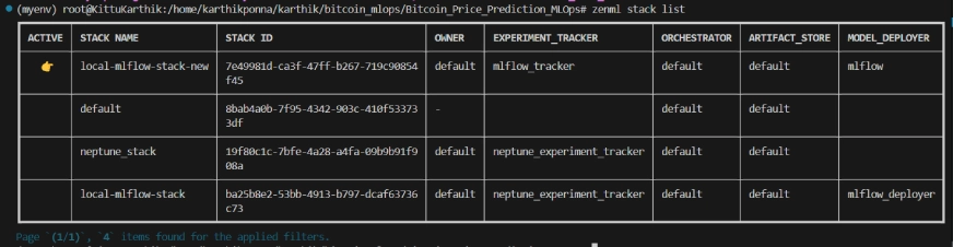
#To view the stack record
zenml stack --listZenML Stack Listing
Challenge Construction
Right here, you may see the structure of the mission. Now let’s talk about it one after the other in nice element.
bitcoin_price_prediction_mlops/        # Challenge listing
├── knowledge/
│   └── administration/
│       ├── api_to_mongodb.py          # Code to fetch knowledge and put it aside to MongoDB
│       └── api.py                     # API-related utility features
│
├── pipelines/
│   ├── deployment_pipeline.py         # Deployment pipeline
│   └── training_pipeline.py           # Coaching pipeline
│
├── saved_models/                      # Listing for storing educated fashions
├── saved_scalers/                     # Listing for storing scalers utilized in knowledge preprocessing
│
├── src/                               # Supply code
│   ├── data_cleaning.py               # Knowledge cleansing and preprocessing
│   ├── data_ingestion.py              # Knowledge ingestion
│   ├── data_splitter.py               # Knowledge splitting
│   ├── feature_engineering.py         # Characteristic engineering
│   ├── model_evaluation.py            # Mannequin analysis
│   └── model_training.py              # Mannequin coaching
│
├── steps/                             # ZenML steps
│   ├── clean_data.py                  # ZenML step for cleansing knowledge
│   ├── data_splitter.py               # ZenML step for knowledge splitting
│   ├── dynamic_importer.py            # ZenML step for importing dynamic knowledge
│   ├── feature_engineering.py         # ZenML step for function engineering
│   ├── ingest_data.py                 # ZenML step for knowledge ingestion
│   ├── model_evaluation.py            # ZenML step for mannequin analysis
│   ├── model_training.py              # ZenML step for coaching the mannequin
│   ├── prediction_service_loader.py   # ZenML step for loading prediction companies
│   ├── predictor.py                   # ZenML step for prediction
│   └── utils.py                       # Utility features for steps
│
├── .env                               # Setting variables file
├── .gitignore                         # Git ignore file
│
├── app.py                             # Streamlit person interface app
│
├── README.md                          # Challenge documentation
├── necessities.txt                   # Listing of required packages
├── run_deployment.py                  # Code for working deployment and prediction pipeline
├── run_pipeline.py                    # Code for working coaching pipeline
└── .zen/                              # ZenML listing (created routinely after ZenML initialization)
Step 4: Knowledge Ingestion
We first ingest knowledge from API to MongoDB and convert it into pandas DataFrame.
import os
import logging
from pymongo import MongoClient
from dotenv import load_dotenv
from zenml import step
import pandas as pd

# Load the .env file
load_dotenv()

# Get MongoDB URI from setting variables
MONGO_URI = os.getenv("MONGO_URI")

def fetch_data_from_mongodb(collection_name:str, database_name:str):
    """
    Fetches knowledge from MongoDB and converts it right into a pandas DataFrame.

    collection_name:
        Identify of the MongoDB assortment to fetch knowledge.
    database_name:
        Identify of the MongoDB database.
    return:
        A pandas DataFrame containing the info
    """
    # Hook up with the MongoDB consumer
    consumer = MongoClient(MONGO_URI)
    db = consumer[database_name]  # Choose the database
    assortment = db[collection_name]  # Choose the gathering

    # Fetch all paperwork from the gathering
    attempt:
        logging.data(f"Fetching knowledge from MongoDB assortment: {collection_name}...")
        knowledge = record(assortment.discover())  # Convert cursor to an inventory of dictionaries

        if not knowledge:
            logging.data("No knowledge discovered within the MongoDB assortment.")


        # Convert the record of dictionaries right into a pandas DataFrame
        df = pd.DataFrame(knowledge)

        # Drop the MongoDB ObjectId area if it exists (optionally available)
        if '_id' in df.columns:
            df = df.drop(columns=['_id'])

        logging.data("Knowledge efficiently fetched and transformed to a DataFrame!")
        return df

    besides Exception as e:
        logging.error(f"An error occurred whereas fetching knowledge: {e}")
        increase e


@step(enable_cache=False)
def ingest_data(collection_name: str = "historical_data", database_name: str = "crypto_data") -> pd.DataFrame:

    logging.data("Began knowledge ingestion course of from MongoDB.")

    attempt:
        # Use the fetch_data_from_mongodb perform to fetch knowledge
        df = fetch_data_from_mongodb(collection_name=collection_name, database_name=database_name)

        if df.empty:
            logging.warning("No knowledge was loaded. Test the gathering identify or the database content material.")
        else:
            logging.data(f"Knowledge ingestion accomplished. Variety of data loaded: {len(df)}.")

        return df

    besides Exception as e:
        logging.error(f"Error whereas studying knowledge from {collection_name} in {database_name}: {e}")
        increase e
we add @step as a decorator to the ingest_data() perform to declare it as a step of our coaching pipeline. In the identical approach, we are going to write code for every step within the mission structure and create the pipeline.
To view how I’ve used the @step decorator, try the GitHub hyperlink beneath (steps folder) to undergo the code for different steps of the pipeline i.e. knowledge cleansing, function engineering, knowledge splitting, mannequin coaching, and mannequin analysis.
Step 5: Knowledge Cleansing
On this step, we are going to create totally different methods for cleansing the ingested knowledge. We are going to drop the undesirable columns and lacking values within the knowledge.
class DataPreprocessor:
    def __init__(self, knowledge: pd.DataFrame):

        self.knowledge = knowledge
        logging.data("DataPreprocessor initialized with knowledge of form: %s", knowledge.form)

    def clean_data(self) -> pd.DataFrame:
        """
        Performs knowledge cleansing by eradicating pointless columns, dropping columns with lacking values,
        and returning the cleaned DataFrame.

        Returns:
            pd.DataFrame: The cleaned DataFrame with pointless and missing-value columns eliminated.
        """
        logging.data("Beginning knowledge cleansing course of.")

        # Drop pointless columns, together with '_id' if it exists
        columns_to_drop = [
            'UNIT', 'TYPE', 'MARKET', 'INSTRUMENT',
            'FIRST_MESSAGE_TIMESTAMP', 'LAST_MESSAGE_TIMESTAMP',
            'FIRST_MESSAGE_VALUE', 'HIGH_MESSAGE_VALUE', 'HIGH_MESSAGE_TIMESTAMP',
            'LOW_MESSAGE_VALUE', 'LOW_MESSAGE_TIMESTAMP', 'LAST_MESSAGE_VALUE',
            'TOTAL_INDEX_UPDATES', 'VOLUME_TOP_TIER', 'QUOTE_VOLUME_TOP_TIER',
            'VOLUME_DIRECT', 'QUOTE_VOLUME_DIRECT', 'VOLUME_TOP_TIER_DIRECT',
            'QUOTE_VOLUME_TOP_TIER_DIRECT', '_id'  # Adding '_id' to the list
        ]
        logging.data("Dropping columns: %s")
        self.knowledge = self.drop_columns(self.knowledge, columns_to_drop)

        # Drop columns the place the variety of lacking values is larger than 0
        logging.data("Dropping columns with lacking values.")
        self.knowledge = self.drop_columns_with_missing_values(self.knowledge)

        logging.data("Knowledge cleansing accomplished. Knowledge form after cleansing: %s", self.knowledge.form)
        return self.knowledge

    def drop_columns(self, knowledge: pd.DataFrame, columns: record) -> pd.DataFrame:
        """
        Drops specified columns from the DataFrame.

        Returns:
            pd.DataFrame: The DataFrame with the desired columns eliminated.
        """
        logging.data("Dropping columns: %s", columns)
        return knowledge.drop(columns=columns, errors="ignore")

    def drop_columns_with_missing_values(self, knowledge: pd.DataFrame) -> pd.DataFrame:
        """
        Drops columns with any lacking values from the DataFrame.

        Parameters:
            knowledge: pd.DataFrame
                The DataFrame from which columns with lacking values will likely be eliminated.

        Returns:
            pd.DataFrame: The DataFrame with columns containing lacking values eliminated.
        """
        missing_columns = knowledge.columns[data.isnull().sum() > 0]
        if not missing_columns.empty:
            logging.data("Columns with lacking values: %s", missing_columns.tolist())
        else:
            logging.data("No columns with lacking values discovered.")
        return knowledge.loc[:, data.isnull().sum() == 0]
Step 6: Characteristic Engineering
This step takes the cleaned knowledge from the sooner data_cleaning step. We’re creating new options like Easy Shifting Common (SMA), Exponential Shifting Common (EMA), and lagged and rolling statistics to seize traits, scale back noise, and make extra dependable predictions from time-series knowledge. Moreover, we scale the options and goal variables utilizing Minmax scaling.
import joblib
import pandas as pd
from abc import ABC, abstractmethod
from sklearn.preprocessing import MinMaxScaler


# Summary class for Characteristic Engineering technique
class FeatureEngineeringStrategy(ABC):
    @abstractmethod
    def generate_features(self, df: pd.DataFrame) -> pd.DataFrame:
        move


# Concrete class for calculating SMA, EMA, RSI, and different options
class TechnicalIndicators(FeatureEngineeringStrategy):
    def generate_features(self, df: pd.DataFrame) -> pd.DataFrame:

        # Calculate SMA, EMA, and RSI
        df['SMA_20'] = df['CLOSE'].rolling(window=20).imply()
        df['SMA_50'] = df['CLOSE'].rolling(window=50).imply()
        df['EMA_20'] = df['CLOSE'].ewm(span=20, regulate=False).imply()

        # Value distinction options
        df['OPEN_CLOSE_diff'] = df['OPEN'] - df['CLOSE']
        df['HIGH_LOW_diff'] = df['HIGH'] - df['LOW']
        df['HIGH_OPEN_diff'] = df['HIGH'] - df['OPEN']
        df['CLOSE_LOW_diff'] = df['CLOSE'] - df['LOW']

        # Lagged options
        df['OPEN_lag1'] = df['OPEN'].shift(1)
        df['CLOSE_lag1'] = df['CLOSE'].shift(1)
        df['HIGH_lag1'] = df['HIGH'].shift(1)
        df['LOW_lag1'] = df['LOW'].shift(1)

        # Rolling statistics
        df['CLOSE_roll_mean_14'] = df['CLOSE'].rolling(window=14).imply()
        df['CLOSE_roll_std_14'] = df['CLOSE'].rolling(window=14).std()

        # Drop rows with lacking values (on account of rolling home windows, shifts)
        df.dropna(inplace=True)

        return df

# Summary class for Scaling technique
class ScalingStrategy(ABC):
    @abstractmethod
    def scale(self, df: pd.DataFrame, options: record, goal: str):
        move

# Concrete class for MinMax Scaling
class MinMaxScaling(ScalingStrategy):
    def scale(self, df: pd.DataFrame, options: record, goal: str):
        """
        Scales the options and goal utilizing MinMaxScaler.

        Parameters:
            df: pd.DataFrame
                The DataFrame containing the options and goal.
            options: record
                Listing of function column names.
            goal: str
                The goal column identify.

        Returns:
            pd.DataFrame, pd.DataFrame: Scaled options and goal
        """
        scaler_X = MinMaxScaler(feature_range=(0, 1))
        scaler_y = MinMaxScaler(feature_range=(0, 1))

        X_scaled = scaler_X.fit_transform(df[features].values)
        y_scaled = scaler_y.fit_transform(df[[target]].values)

        joblib.dump(scaler_X, 'saved_scalers/scaler_X.pkl')
        joblib.dump(scaler_y, 'saved_scalers/scaler_y.pkl')

        return X_scaled, y_scaled, scaler_y


# FeatureEngineeringContext: It will use the Technique Sample
class FeatureEngineering:
    def __init__(self, feature_strategy: FeatureEngineeringStrategy, scaling_strategy: ScalingStrategy):
        self.feature_strategy = feature_strategy
        self.scaling_strategy = scaling_strategy

    def process_features(self, df: pd.DataFrame, options: record, goal: str):
        # Generate options utilizing the offered technique
        df_with_features = self.feature_strategy.generate_features(df)

        # Scale options and goal utilizing the offered technique
        X_scaled, y_scaled, scaler_y = self.scaling_strategy.scale(df_with_features, options, goal)

        return df_with_features, X_scaled, y_scaled, scaler_y
Step 7: Knowledge Splitting
Now, we cut up the processed knowledge into coaching and testing datasets within the ratio of 80:20.
import logging
from abc import ABC, abstractmethod
import numpy as np
from sklearn.model_selection import train_test_split

# Arrange logging configuration
logging.basicConfig(degree=logging.INFO, format="%(asctime)s - %(levelname)s - %(message)s")

# Summary Base Class for Knowledge Splitting Technique
class DataSplittingStrategy(ABC):
    @abstractmethod
    def split_data(self, X: np.ndarray, y: np.ndarray):
        move

# Concrete Technique for Easy Practice-Take a look at Break up
class SimpleTrainTestSplitStrategy(DataSplittingStrategy):
    def __init__(self, test_size=0.2, random_state=42):

        self.test_size = test_size
        self.random_state = random_state

    def split_data(self, X: np.ndarray, y: np.ndarray):

        logging.data("Performing easy train-test cut up.")
        X_train, X_test, y_train, y_test = train_test_split(
            X, y, test_size=self.test_size, random_state=self.random_state
        )
        logging.data("Practice-test cut up accomplished.")
        return X_train, X_test, y_train, y_test

# Context Class for Knowledge Splitting
class DataSplitter:
    def __init__(self, technique: DataSplittingStrategy):

        self._strategy = technique

    def set_strategy(self, technique: DataSplittingStrategy):

        logging.data("Switching knowledge splitting technique.")
        self._strategy = technique

    def cut up(self, X: np.ndarray, y: np.ndarray):

        logging.data("Splitting knowledge utilizing the chosen technique.")
        return self._strategy.split_data(X, y)
Step 8: Mannequin Coaching
On this step, we practice the LSTM mannequin with early stopping to forestall overfitting, and by utilizing MLflow’s automated logging to trace our mannequin and experiments and save the educated mannequin as lstm_model.keras.
import numpy as np
import logging
import mlflow
from tensorflow.keras.fashions import Sequential
from tensorflow.keras.layers import Enter, LSTM, Dropout, Dense
from tensorflow.keras.regularizers import l2
from tensorflow.keras.callbacks import EarlyStopping
from typing import Any

# Summary Base Class for Mannequin Constructing Technique
class ModelBuildingStrategy:

    def build_and_train_model(self, X_train: np.ndarray, y_train: np.ndarray, fine_tuning: bool = False) -> Any:
        move

# Concrete Technique for LSTM Mannequin
class LSTMModelStrategy(ModelBuildingStrategy):
    def build_and_train_model(self, X_train: np.ndarray, y_train: np.ndarray, fine_tuning: bool = False) -> Any:
        """
        Trains an LSTM mannequin on the offered coaching knowledge.

        Parameters:
            X_train (np.ndarray): The coaching knowledge options.
            y_train (np.ndarray): The coaching knowledge labels/goal.
            fine_tuning (bool): Not relevant for LSTM, defaults to False.

        Returns:
            tf.keras.Mannequin: A educated LSTM mannequin.
        """
        logging.data("Constructing and coaching the LSTM mannequin.")

        # MLflow autologging
        mlflow.tensorflow.autolog()

        logging.data(f"form of X_train:{X_train.form}")

        # LSTM Mannequin Definition
        mannequin = Sequential()
        mannequin.add(Enter(form=(X_train.form[1], X_train.form[2])))

        mannequin.add(LSTM(items=50, return_sequences=True, kernel_regularizer=l2(0.01)))
        mannequin.add(Dropout(0.3))
        mannequin.add(LSTM(items=50, return_sequences=False))
        mannequin.add(Dropout(0.2))
        mannequin.add(Dense(items=1))  # Modify the variety of items primarily based in your output (e.g., regression or classification)

        # Compiling the mannequin
        mannequin.compile(optimizer="adam", loss="mean_squared_error")

        # Early stopping to keep away from overfitting
        early_stopping = EarlyStopping(monitor="val_loss", persistence=10, restore_best_weights=True)

        # Match the mannequin
        historical past = mannequin.match(
            X_train,
            y_train,
            epochs=50,
            batch_size=32,
            validation_split=0.1,
            callbacks=[early_stopping],
            verbose=1
        )

        mlflow.log_metric("final_loss", historical past.historical past["loss"][-1])

        # Saving the educated mannequin
        mannequin.save("saved_models/lstm_model.keras")
        logging.data("LSTM mannequin educated and saved.")

        return mannequin

# Context Class for Mannequin Constructing Technique
class ModelBuilder:
    def __init__(self, technique: ModelBuildingStrategy):
        self._strategy = technique

    def set_strategy(self, technique: ModelBuildingStrategy):
        self._strategy = technique

    def practice(self, X_train: np.ndarray, y_train: np.ndarray, fine_tuning: bool = False) -> Any:
        return self._strategy.build_and_train_model(X_train, y_train, fine_tuning)
Step 9: Mannequin Analysis
As it is a regression drawback, we’re utilizing analysis metrics like Imply Squared Error (MSE), Root Imply Squared Error (MSE), Imply Absolute Error (MAE), and R-squared.
import logging
import numpy as np
from abc import ABC, abstractmethod
from sklearn.preprocessing import MinMaxScaler
from sklearn.metrics import mean_squared_error, mean_absolute_error, r2_score
from typing import Dict

# Setup logging configuration
logging.basicConfig(degree=logging.INFO, format="%(asctime)s - %(levelname)s - %(message)s")

# Summary Base Class for Mannequin Analysis Technique
class ModelEvaluationStrategy(ABC):
    @abstractmethod
    def evaluate_model(self, mannequin, X_test, y_test, scaler_y) -> Dict[str, float]:
        move

# Concrete Technique for Regression Mannequin Analysis
class RegressionModelEvaluationStrategy(ModelEvaluationStrategy):
    def evaluate_model(self, mannequin, X_test, y_test, scaler_y) -> Dict[str, float]:
        # Predict the info
        y_pred = mannequin.predict(X_test)

        # Guarantee y_test and y_pred are reshaped into 2D arrays for inverse transformation
        y_test_reshaped = y_test.reshape(-1, 1)
        y_pred_reshaped = y_pred.reshape(-1, 1)

        # Inverse rework the scaled predictions and true values
        y_pred_rescaled = scaler_y.inverse_transform(y_pred_reshaped)
        y_test_rescaled = scaler_y.inverse_transform(y_test_reshaped)

        # Flatten the arrays to make sure they're 1D
        y_pred_rescaled = y_pred_rescaled.flatten()
        y_test_rescaled = y_test_rescaled.flatten()

        # Calculate analysis metrics
        mse = mean_squared_error(y_test_rescaled, y_pred_rescaled)
        rmse = np.sqrt(mse)
        mae = mean_absolute_error(y_test_rescaled, y_pred_rescaled)
        r2 = r2_score(y_test_rescaled, y_pred_rescaled)

        # Logging the metrics
        logging.data("Calculating analysis metrics.")
        metrics = {
            "Imply Squared Error - MSE": mse,
            "Root Imply Squared Error - RMSE": rmse,
            "Imply Absolute Error - MAE": mae,
            "R-squared - R²": r2
        }

        logging.data(f"Mannequin Analysis Metrics: {metrics}")
        return metrics

# Context Class for Mannequin Analysis
class ModelEvaluator:
    def __init__(self, technique: ModelEvaluationStrategy):

        self._strategy = technique

    def set_strategy(self, technique: ModelEvaluationStrategy):

        logging.data("Switching mannequin analysis technique.")
        self._strategy = technique

    def consider(self, mannequin, X_test, y_test, scaler_y) -> Dict[str, float]:

        logging.data("Evaluating the mannequin utilizing the chosen technique.")
        return self._strategy.evaluate_model(mannequin, X_test, y_test, scaler_y)
Now we will manage all of the above steps right into a pipeline. Let’s create a brand new file training_pipeline.py.
from zenml import Mannequin, pipeline

@pipeline(
    mannequin=Mannequin(
        # The identify uniquely identifies this mannequin
        identify="bitcoin_price_predictor"
    ),
)
def ml_pipeline():
    # Knowledge Ingestion Step
    raw_data = ingest_data()
    # Knowledge Cleansing Step
    cleaned_data = clean_data(raw_data)
    # Characteristic Engineering Step
    transformed_data, X_scaled, y_scaled, scaler_y = feature_engineering_step(
        cleaned_data
    )
    # Knowledge Splitting
    X_train, X_test, y_train, y_test = data_splitter_step(X_scaled=X_scaled, y_scaled=y_scaled)
    # Mannequin Coaching
    mannequin = model_training_step(X_train, y_train)
    # Mannequin Analysis
    evaluator = model_evaluation_step(mannequin, X_test=X_test, y_test=y_test, scaler_y= scaler_y)

    return evaluator
Right here, @pipeline decorator is used to outline the perform ml_pipeline() as a pipeline in ZenML.
To view the dashboard for the coaching pipeline, merely run the run_pipeline.py script. Let’s create a run_pipeline.py file.
import click on
from pipelines.training_pipeline import ml_pipeline

@click on.command()
def fundamental():
    run = ml_pipeline()

if __name__=="__main__":
    fundamental()
Now we’ve got accomplished creating the pipeline. Run the command beneath to view the pipeline dashboard.
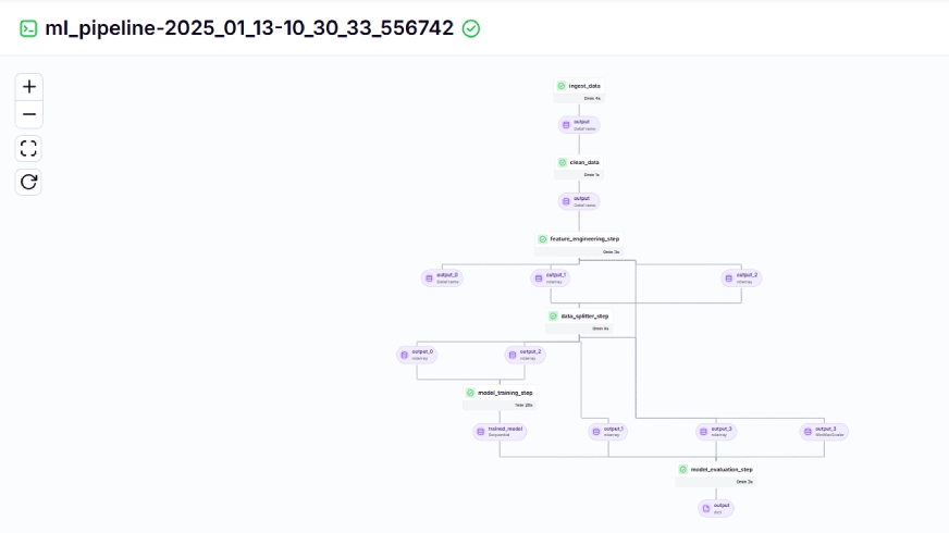
python run_pipeline.pyAfter working the above command it can return the monitoring dashboard URL, which appears like this.
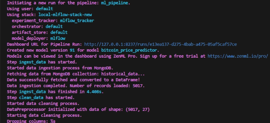
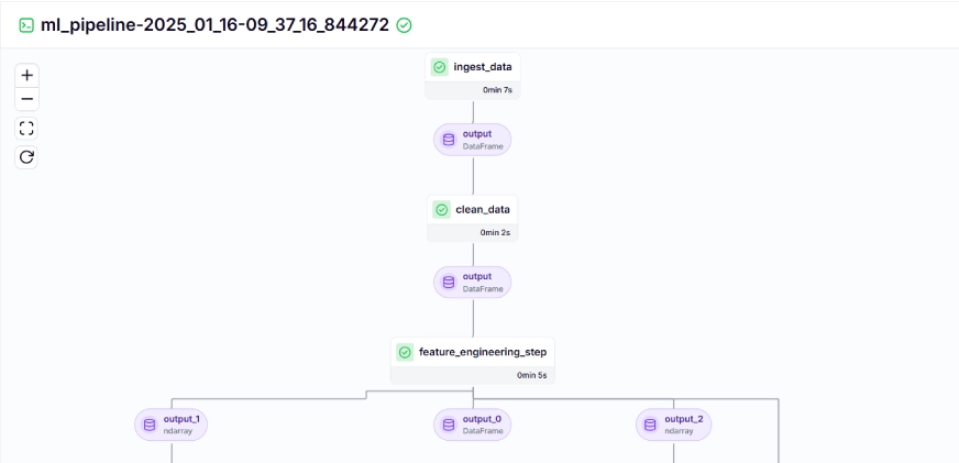
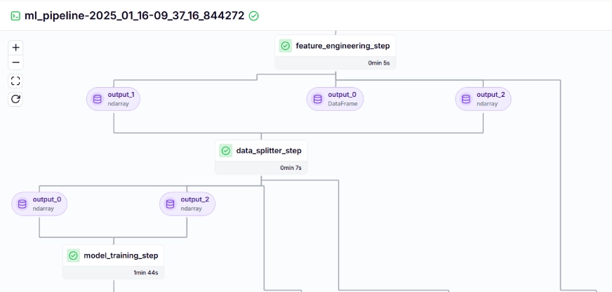
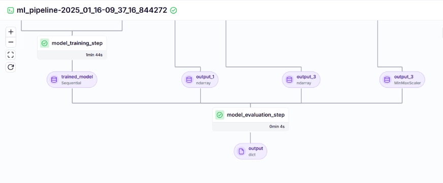
The coaching pipeline appears like this within the dashboard, given beneath:
Step 10: Mannequin Deployment
Until now we’ve got constructed the mannequin and the pipelines. Now let’s push the pipeline into manufacturing the place customers could make predictions.
Steady Deployment Pipeline
from zenml.integrations.mlflow.steps import mlflow_model_deployer_step

@pipeline
def continuous_deployment_pipeline():
    trained_model = ml_pipeline()
    mlflow_model_deployer_step(staff=3,deploy_decision=True,mannequin=trained_model,)
This pipeline is answerable for repeatedly deploying educated fashions. It first runs the ml_pipeline() from the training_pipeline.py file to coach the mannequin, then makes use of the Mlflow Mannequin Deployer to deploy the educated mannequin utilizing the continuous_deployment_pipeline().
Inference Pipeline
We use an inference pipeline to make predictions on the brand new knowledge, utilizing the deployed mannequin. Let’s check out how we applied this pipeline in our mission.
@pipeline
def inference_pipeline(enable_cache=True):
    """Run a batch inference job with knowledge loaded from an API."""
    batch_data = dynamic_importer()
    model_deployment_service = prediction_service_loader(
        pipeline_name="continuous_deployment_pipeline",
        step_name="mlflow_model_deployer_step",
    )
    predictor(service=model_deployment_service, input_data=batch_data)
Allow us to see about every of the features known as within the inference pipeline beneath:
dynamic_importer()
This perform masses the brand new knowledge, performs knowledge processing, and returns the info.
@step
def dynamic_importer() -> str:
    """Dynamically imports knowledge for testing the mannequin with anticipated columns."""

    attempt:
        knowledge = {
            'OPEN': [0.98712925, 1.],'HIGH': [0.57191823, 0.55107652],'LOW': [1., 0.94728144],'VOLUME': [0.18186191, 0.],'SMA_20': [0.90819243, 1.],'SMA_50': [0.90214911, 1.],'EMA_20': [0.89735654, 1.],'OPEN_CLOSE_diff': [0.61751032, 0.57706902],'HIGH_LOW_diff': [0.01406254, 0.02980481],
            'HIGH_OPEN_diff': [0.13382262, 0.09172282],
            'CLOSE_LOW_diff': [0.14140073, 0.28523136],'OPEN_lag1': [0.64467168, 1.],
            'CLOSE_lag1': [0.98712925, 1.],
            'HIGH_lag1': [0.77019885, 0.57191823],
            'LOW_lag1': [0.64465093, 1.],
            'CLOSE_roll_mean_14': [0.94042809, 1.],'CLOSE_roll_std_14': [0.22060724, 0.35396897],
        }

        df = pd.DataFrame(knowledge)
        data_array = df.iloc[0].values
        reshaped_data = data_array.reshape((1, 1, data_array.form[0]))  # Single pattern, 1 time step, 17 options

        logging.data(f"Reshaped Knowledge: {reshaped_data.form}")

        json_data = pd.DataFrame(reshaped_data.reshape((reshaped_data.form[0], reshaped_data.form[2]))).to_json(orient="cut up")

        return json_data

    besides Exception as e:
        logging.error(f"Error throughout importing knowledge from dynamic importer: {e}")
        increase e
prediction_service_loader()
This perform is adorned with @step. We load the deployment service w.r.t the deployed mannequin primarily based on the pipeline_name, and step_name, the place our deployed mannequin is able to course of prediction queries for the brand new knowledge.
The road existing_services=mlflow_model_deployer_component.find_model_server() searches for an accessible deployment service primarily based on the given parameters like pipeline identify and pipeline step identify. If no companies can be found, it signifies that the deployment pipeline has both not been carried out or encountered an issue with the deployment pipeline, so it throws a RuntimeError.
@step(enable_cache=False)
def prediction_service_loader(pipeline_name: str, step_name: str) -> MLFlowDeploymentService:
    model_deployer = MLFlowModelDeployer.get_active_model_deployer()

    existing_services = model_deployer.find_model_server(
        pipeline_name=pipeline_name,
        pipeline_step_name=step_name,
    )

    if not existing_services:
        increase RuntimeError(
            f"No MLflow prediction service deployed by the "
            f"{step_name} step within the {pipeline_name} "
            f"pipeline is at present "
            f"working."
        )
    return existing_services[0]
predictor()
The perform takes within the MLFlow-deployed mannequin by way of the MLFlowDeploymentService and the brand new knowledge. The info is processed additional to match the anticipated format of the mannequin to make real-time inferences.
@step(enable_cache=False)
def predictor(
    service: MLFlowDeploymentService,
    input_data: str,
) -> np.ndarray:

    service.begin(timeout=10)

    attempt:
        knowledge = json.masses(input_data)
        knowledge.pop("columns", None)
        knowledge.pop("index", None)

        if isinstance(knowledge["data"], record):
            data_array = np.array(knowledge["data"])
        else:
            increase ValueError("The info format is inaccurate, anticipated an inventory beneath 'knowledge'.")

        if data_array.form != (1, 1, 17):
            data_array = data_array.reshape((1, 1, 17))  # Modify the form as wanted

        attempt:
            prediction = service.predict(data_array)
        besides Exception as e:
            increase ValueError(f"Prediction failed: {e}")
        return prediction

    besides json.JSONDecodeError:
        increase ValueError("Invalid JSON format within the enter knowledge.")
    besides KeyError as e:
        increase ValueError(f"Lacking anticipated key in enter knowledge: {e}")
    besides Exception as e:
        increase ValueError(f"An error occurred throughout knowledge processing: {e}")
To visualise the continual deployment and inference pipeline, we have to run the run_deployment.py script, the place the deployment and prediction configurations will likely be outlined. (Please examine the run_deployment.py code within the GitHub given beneath).
@click on.choice(
    "--config",
    sort=click on.Selection([DEPLOY, PREDICT, DEPLOY_AND_PREDICT]),
    default=DEPLOY_AND_PREDICT,
    assist="Optionally you may select to solely run the deployment "
    "pipeline to coach and deploy a mannequin (`deploy`), or to "
    "solely run a prediction in opposition to the deployed mannequin "
    "(`predict`). By default each will likely be run "
    "(`deploy_and_predict`).",
)
Now let’s run the run_deployment.py file to see the dashboard of the continual deployment pipeline and inference pipeline.
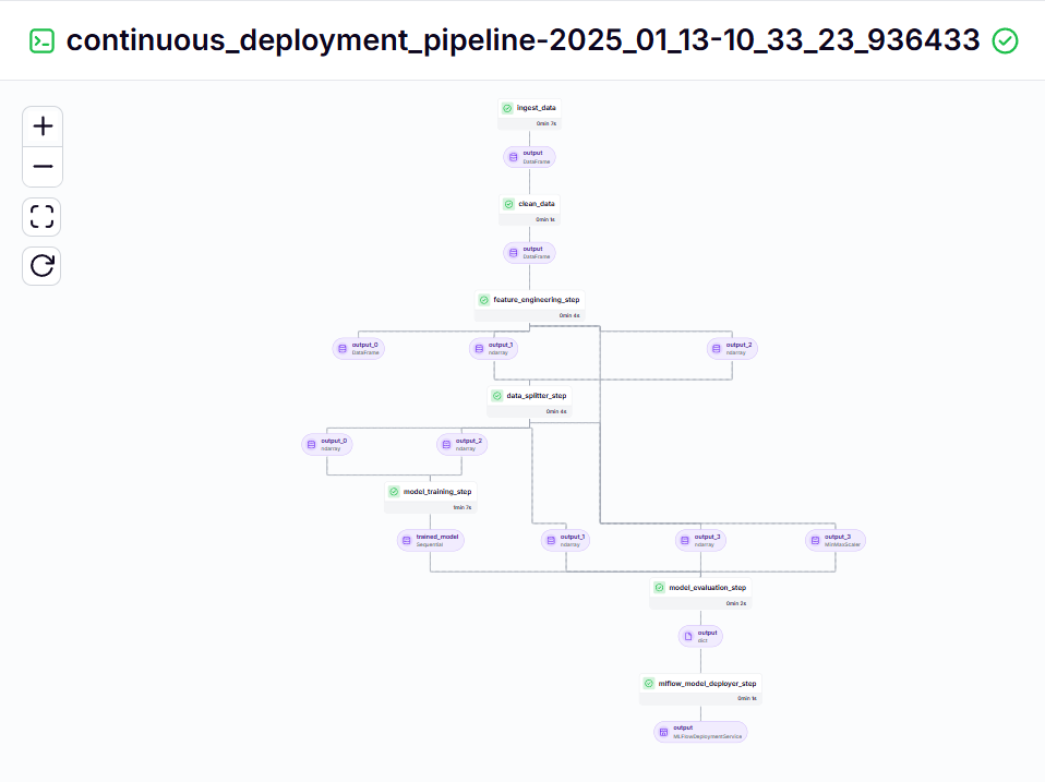
python run_deployment.pySteady Deployment Pipeline – Output
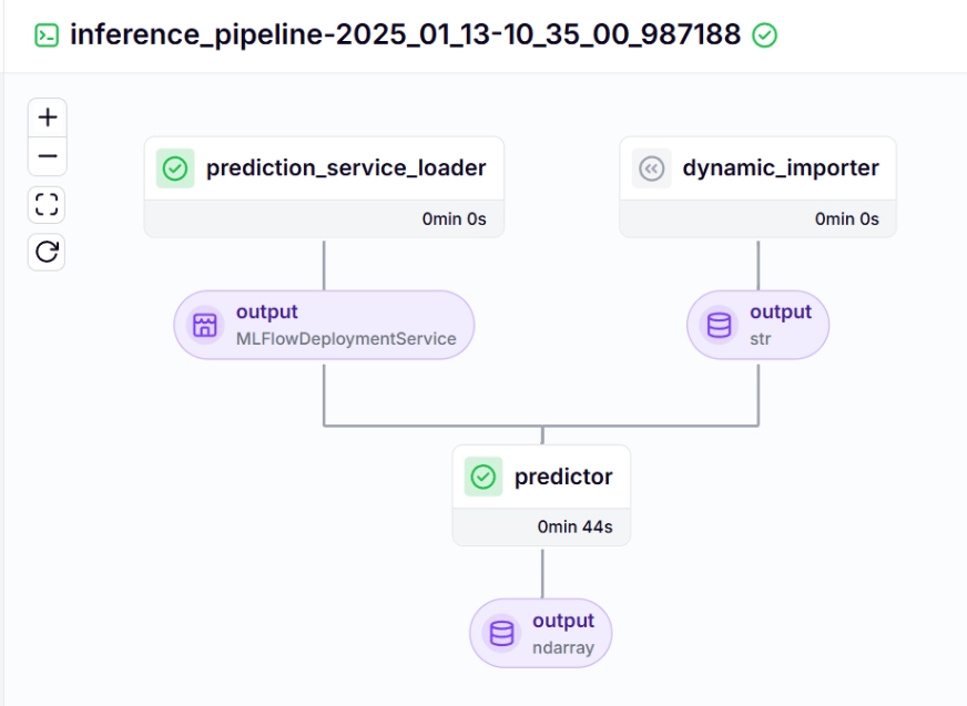
Inference Pipeline – Output
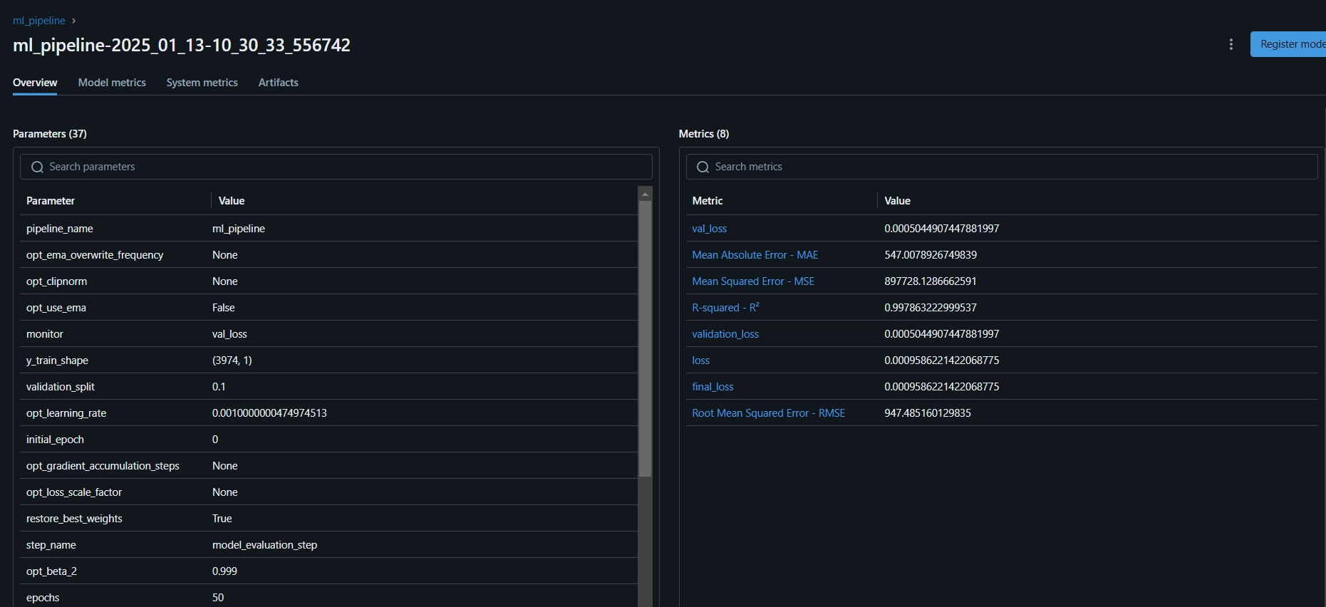
After working the run_deployment.py file you may see the MLflow dashboard hyperlink which appears like this.
mlflow ui --backend-store-uri file:/root/.config/zenml/local_stores/cd1eb06a-179a-4f83-9bae-9b9a5b1bd27f/mlrunsNow you must copy and paste the above MLflow UI hyperlink in your command line and run it.
Right here is the MLflow dashboard, the place you may see the analysis metrics and mannequin parameters:
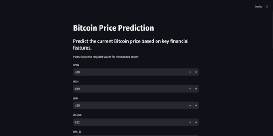
Step 11: Constructing the Streamlit App
Streamlit is an incredible open-source, Python-based framework, used to create interactive UI’s, we will use Streamlit to construct internet apps shortly, with out realizing backend or frontend improvement. First, we have to set up Streamlit on our system.
#Set up streamlit in our native PC
pip set up streamlit

#To run the streamlit native internet server
streamlit run app.py
Once more, you could find the code on GitHub for the Streamlit app.
Right here’s the GitHub Code and Video Rationalization of the Challenge on your higher understanding.
Conclusion
On this article, we’ve got efficiently constructed an end-to-end, production-ready Bitcoin Value Prediction MLOps mission. From buying knowledge by way of an API and preprocessing it to mannequin coaching, analysis, and deployment, our mission highlights the crucial function of MLOps in connecting improvement with manufacturing. We’re one step nearer to shaping the way forward for predicting Bitcoin costs in actual time. APIs present clean entry to exterior knowledge, like Bitcoin worth knowledge from the CCData API, eliminating the necessity for a pre-existing dataset.
Key Takeaways
- APIs allow seamless entry to exterior knowledge, like Bitcoin worth knowledge from CCData API, eliminating the necessity for a pre-existing dataset.
- ZenML and MLflow are sturdy instruments that facilitate the event, monitoring, and deployment of machine studying fashions in real-world functions.
- We’ve adopted finest practices by correctly performing knowledge ingestion, cleansing, function engineering, mannequin coaching, and analysis.
- Steady deployment and inference pipelines are important for guaranteeing that fashions stay environment friendly and accessible in manufacturing environments.
Often Requested Questions
A. Sure, ZenML is a completely open-source MLOps framework that makes the transition from native improvement to manufacturing pipelines as simple as 1 line of code.
A. MLflow makes machine studying improvement simpler by providing instruments for monitoring experiments, versioning fashions, and deploying them.
A. This can be a widespread error you’ll face within the mission. Simply run `zenml logout –native` then `zenml clear`, after which `zenml login –native`, once more run the pipeline. Will probably be resolved.
Hello! I am Karthik Ponna, a Machine Studying Engineer at Antern. I am deeply enthusiastic about exploring the fields of AI and Knowledge Science, as they continuously evolve and form the longer term. I imagine writing blogs is a good way to not solely improve my abilities and solidify my understanding but in addition to share my data and insights with others locally. This helps me join with like-minded people who share a curiosity for expertise and innovation.
Login to proceed studying and revel in expert-curated content material.