
On this article, you’ll learn to flip a uncooked time sequence right into a supervised studying dataset and use resolution tree-based fashions to forecast future values.
Subjects we’ll cowl embrace:
- Engineering lag options and rolling statistics from a univariate sequence.
- Making ready a chronological practice/take a look at break up and becoming a choice tree regressor.
- Evaluating with MAE and avoiding knowledge leakage with correct characteristic design.
Let’s not waste any extra time.
Forecasting the Future with Tree-Primarily based Fashions for Time Sequence
Picture by Editor
Introduction
Choice tree-based fashions in machine studying are often used for a variety of predictive duties corresponding to classification and regression, sometimes on structured, tabular knowledge. Nevertheless, when mixed with the precise knowledge processing and have extraction approaches, resolution bushes additionally turn out to be a robust predictive device for different knowledge codecs like textual content, photos, or time sequence.
This text demonstrates how resolution bushes can be utilized to carry out time sequence forecasting. Extra particularly, we present the best way to extract important options from uncooked time sequence — corresponding to lagged options and rolling statistics — and leverage this structured info to carry out the aforementioned predictive duties by coaching resolution tree-based fashions.
Constructing Choice Bushes for Time Sequence Forecasting
On this hands-on tutorial, we’ll use the month-to-month airline passengers dataset obtainable at no cost within the sktime library. It is a small univariate time sequence dataset containing month-to-month passenger numbers for an airline listed by year-month, between 1949 and 1960.
Let’s begin by loading the dataset — chances are you’ll must pip set up sktime first when you haven’t used the library earlier than:
|
import pandas as pd from sktime.datasets import load_airline
y = load_airline() y.head() |
Since this can be a univariate time sequence, it’s managed as a one-dimensional pandas Sequence listed by date (month-year), somewhat than a two-dimensional DataFrame object.
To extract related options from our time sequence and switch it into a totally structured dataset, we outline a customized operate referred to as make_lagged_df_with_rolling, which takes the uncooked time sequence as enter, plus two key phrase arguments: lags and roll_window, which we’ll clarify shortly:
|
def make_lagged_df_with_rolling(sequence, lags=12, roll_window=3): df = pd.DataFrame({“y”: sequence})
for lag in vary(1, lags+1): df[f“lag_{lag}”] = df[“y”].shift(lag)
df[f“roll_mean_{roll_window}”] = df[“y”].shift(1).rolling(roll_window).imply() df[f“roll_std_{roll_window}”] = df[“y”].shift(1).rolling(roll_window).std()
return df.dropna()
df_features = make_lagged_df_with_rolling(y, lags=12, roll_window=3) df_features.head() |
Time to revisit the above code and see what occurred contained in the operate:
- We first pressure our univariate time sequence to turn out to be a pandas
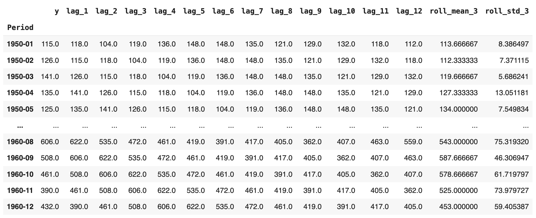
DataFrame, as we’ll shortly broaden it with a number of further options. - We incorporate lagged options; i.e., given a selected passenger worth at a timestamp, we accumulate the earlier values from previous months. In our state of affairs, at time t, we embrace all consecutive readings from t-1 as much as t-12 months earlier, as proven within the picture under. For January 1950, for example, we now have each the unique passenger numbers and the equal values for the earlier 12 months added throughout 12 further attributes, in reverse temporal order.
- Lastly, we add two extra attributes containing the rolling common and rolling commonplace deviation, respectively, spanning three months. That’s, given a month-to-month studying of passenger numbers, we calculate the common or commonplace deviation of the newest n = 3 months excluding the present month (see using
.shift(1)earlier than the.rolling()name), which prevents look-ahead leakage.
The ensuing enriched dataset ought to seem like this:
After that, coaching and testing the choice tree is easy and executed as normal with scikit-learn fashions. The one side to remember is: what shall be our goal variable to foretell? In fact, we wish to forecast “unknown” values of passenger numbers at a given month based mostly on the remainder of the options extracted. Subsequently, the unique time sequence variable turns into our goal label. Additionally, be sure to select the DecisionTreeRegressor, as we’re targeted on numerical predictions on this state of affairs, not classifications:
Partitioning the dataset into coaching and take a look at, and separating the labels from predictor options:
|
train_size = int(len(df_features) * 0.8) practice, take a look at = df_features.iloc[:train_size], df_features.iloc[train_size:]
X_train, y_train = practice.drop(“y”, axis=1), practice[“y”] X_test, y_test = take a look at.drop(“y”, axis=1), take a look at[“y”] |
Coaching and evaluating the choice tree error (MAE):
|
from sklearn.tree import DecisionTreeRegressor from sklearn.metrics import mean_absolute_error
dt_reg = DecisionTreeRegressor(max_depth=5, random_state=42) dt_reg.match(X_train, y_train) y_pred = dt_reg.predict(X_test)
print(“Forecasting:”) print(“MAE:”, mean_absolute_error(y_test, y_pred)) |
In a single run, the ensuing error was MAE ≈ 45.32. That isn’t dangerous, contemplating that month-to-month passenger numbers within the dataset are within the a number of a whole bunch; after all, there may be room for enchancment by utilizing ensembles, extracting further options, tuning hyperparameters, or exploring various fashions.
A last takeaway: not like conventional time sequence forecasting strategies, which predict a future or unknown worth based mostly solely on previous values of the identical variable, the choice tree we constructed predicts that worth based mostly on different options we created. In observe, it’s typically efficient to mix each approaches with two totally different mannequin varieties to acquire extra strong predictions.
Wrapping Up
This text confirmed the best way to practice resolution tree fashions able to coping with time sequence knowledge by extracting options from them. Beginning with a uncooked univariate time sequence of month-to-month passenger numbers for an airline, we extracted lagged options and rolling statistics to behave as predictor attributes and carried out forecasting by way of a educated resolution tree.