What’s Beam Search in NLP Decoding?

Beam search is a robust decoding algorithm extensively utilized in pure language processing (NLP) and machine studying. It’s particularly essential in sequence era duties akin to textual content era, machine translation, and summarization. Beam search balances between exploring the search house effectively and producing high-quality output. On this weblog, we are going to dive deep into the workings of beam search, its significance in decoding, and an implementation whereas exploring its real-world purposes and challenges.

Studying Targets

• Perceive the idea and dealing mechanism of the beam search algorithm in sequence decoding duties.
• Be taught the importance of beam width and the way it balances exploration and effectivity in search areas.
• Discover the sensible implementation of beam search utilizing Python with step-by-step steerage.
• Analyze real-world purposes and challenges related to beam search in NLP duties.
• Achieve insights into the benefits of beam search over different decoding algorithms like grasping search.

This text was printed as part of the Information Science Blogathon.

What’s Beam Search?

Beam search is a heuristic search algorithm used to decode sequences from fashions akin to transformers, LSTMs, and different sequence-to-sequence architectures. It generates textual content by sustaining a set quantity (“beam width”) of essentially the most possible sequences at every step. Not like grasping search, which solely picks the more than likely subsequent token, beam search considers a number of hypotheses without delay. This ensures that the ultimate sequence will not be solely fluent but in addition globally optimum when it comes to mannequin confidence.

For instance, in machine translation, there is likely to be a number of legitimate methods to translate a sentence. Beam search permits the mannequin to discover these prospects by retaining observe of a number of candidate translations concurrently.

How Does Beam Search Work?

Beam search works by exploring a graph the place nodes signify tokens and edges signify possibilities of transitioning from one token to a different. At every step:

• The algorithm selects the top-k most possible tokens primarily based on the mannequin’s output logits (likelihood distribution).
• It expands these tokens into sequences, calculates their cumulative possibilities, and retains the top-k sequences for the subsequent step.
• This course of continues till a stopping situation is met, akin to reaching a particular end-of-sequence token or a predefined size.

Idea of Beam Width

The “beam width” determines what number of candidate sequences are retained at every step. A bigger beam width permits for exploring extra sequences however will increase computational value. Conversely, a smaller beam width is quicker however dangers lacking higher sequences resulting from restricted exploration.

Why Beam Search is Vital in Decoding?

Beam search is important in decoding for a number of causes:

• Improved Sequence High quality: By exploring a number of hypotheses, beam search ensures that the generated sequence is globally optimum quite than being caught in an area optimum.
• Dealing with Ambiguities: Many NLP duties contain ambiguities, akin to a number of legitimate translations or interpretations. Beam search helps discover these prospects and choose the perfect one.
• Effectivity: In comparison with exhaustive search, beam search is computationally environment friendly whereas nonetheless exploring a good portion of the search house.
• Flexibility: Beam search will be tailored to numerous duties and sampling methods, making it a flexible selection for sequence decoding.

Sensible Implementation of Beam Search

Beneath is a sensible instance of beam search implementation. The algorithm builds a search tree, evaluates cumulative scores, and selects the perfect sequence:

Step 1: Set up and Import Dependencies

# Set up transformers and graphviz
!sudo apt-get set up graphviz graphviz-dev
!pip set up transformers pygraphviz

from transformers import GPT2LMHeadModel, GPT2Tokenizer
import torch
import matplotlib.pyplot as plt
import networkx as nx
import numpy as np
from matplotlib.colours import LinearSegmentedColormap
from tqdm import tqdm
import matplotlib.colours as mcolors

System Instructions: Installs required libraries for graph era (graphviz) and Python packages (transformers and pygraphviz).

Imported Libraries:

• transformers: To load GPT-2 for textual content era.
• torch: For dealing with tensors and working computations on the mannequin.
• matplotlib.pyplot: To plot the beam search graph.
• networkx: For developing and managing the tree-like graph representing beam search paths.
• tqdm: To show a progress bar whereas processing the graph.
• numpy and matplotlib.colours: For working with numerical information and colour mappings in visualizations.

Output:

Step 2: Mannequin and Tokenizer Setup

# Load mannequin and tokenizer
system="cuda" if torch.cuda.is_available() else 'cpu'
mannequin = GPT2LMHeadModel.from_pretrained('gpt2').to(system)
tokenizer = GPT2Tokenizer.from_pretrained('gpt2')
mannequin.eval()

• Detects whether or not a GPU (cuda) is out there, as it could possibly speed up computations. Defaults to cpu if no GPU is discovered.
• Hundreds the pre-trained GPT-2 language mannequin and its tokenizer from Hugging Face’s transformers library.
• Strikes the mannequin to the suitable system (cuda or cpu).
• Units the mannequin to analysis mode with mannequin.eval() to disable options like dropout, that are solely wanted throughout coaching.

Output:

Step 3: Encode Enter Textual content

# Enter textual content
textual content = "I've a dream"
input_ids = tokenizer.encode(textual content, return_tensors="pt").to(system)

• Defines the enter textual content “I’ve a dream”.
• Encodes the textual content into token IDs utilizing the tokenizer, returning a tensor (return_tensors=’pt’).
• Strikes the enter tensor to the suitable system (cuda or cpu).

Step 4: Outline Helper Operate: Log Likelihood

def get_log_prob(logits, token_id):
    possibilities = torch.nn.purposeful.softmax(logits, dim=-1)
    log_probabilities = torch.log(possibilities)
    return log_probabilities[token_id].merchandise()

• Applies the softmax operate to transform logits into possibilities (distribution over vocabulary).
• Takes the pure logarithm of those possibilities to get log possibilities.
• Returns the log likelihood equivalent to the given token.

Step 5: Outline Recursive Beam Search

Implements recursive beam seek for textual content era utilizing the GPT-2 mannequin.

def beam_search(input_ids, node, bar, size, beams, temperature=1.0):
    if size == 0:
        return

    outputs = mannequin(input_ids)
    predictions = outputs.logits

    # Get logits for the subsequent token
    logits = predictions[0, -1, :]
    top_token_ids = torch.topk(logits, beams).indices

    for j, token_id in enumerate(top_token_ids):
        bar.replace(1)

        # Compute the rating of the anticipated token
        token_score = get_log_prob(logits, token_id)
        cumulative_score = graph.nodes[node]['cumscore'] + token_score

        # Add the anticipated token to the checklist of enter ids
        new_input_ids = torch.cat([input_ids, token_id.unsqueeze(0).unsqueeze(0)], dim=-1)

        # Add node and edge to graph
        token = tokenizer.decode(token_id, skip_special_tokens=True)
        current_node = checklist(graph.successors(node))[j]
        graph.nodes[current_node]['tokenscore'] = np.exp(token_score) * 100
        graph.nodes[current_node]['cumscore'] = cumulative_score
        graph.nodes[current_node]['sequencescore'] = cumulative_score / len(new_input_ids.squeeze())
        graph.nodes[current_node]['token'] = token + f"_{size}_{j}"

        # Recursive name
        beam_search(new_input_ids, current_node, bar, size - 1, beams, temperature)

• Base Case: Stops recursion when size reaches 0 (no extra tokens to foretell).
• Mannequin Prediction: Passes input_ids via GPT-2 to get logits for the subsequent token.
• High Beams: Selects the beams more than likely tokens utilizing torch.topk().
• Token Scoring: Evaluates token possibilities to find out the perfect sequences.
• Lengthen Enter: Appends the chosen token to input_ids for additional exploration.
• Replace Graph: Tracks progress by increasing the search tree with new tokens.
• Recursive Name: Repeats the method for every beam (beams branches).

Step 6: Retrieve Greatest Sequence

Finds the perfect sequence generated throughout beam search primarily based on cumulative scores.

def get_best_sequence(G):
    # Discover all leaf nodes
    leaf_nodes = [node for node in G.nodes if G.out_degree(node) == 0]

    # Discover the perfect leaf node primarily based on sequence rating
    max_score_node = max(leaf_nodes, key=lambda n: G.nodes[n]['sequencescore'])
    max_score = G.nodes[max_score_node]['sequencescore']

    # Retrieve the trail from root to this node
    path = nx.shortest_path(G, supply=0, goal=max_score_node)

    # Assemble the sequence
    sequence = "".be part of([G.nodes[node]['token'].break up('_')[0] for node in path])
    return sequence, max_score

• Identifies all leaf nodes (nodes with no outgoing edges).
• Finds the perfect leaf node (highest sequencescore).
• Retrieves the trail from the foundation node (begin) to the perfect node.
• Extracts and joins tokens alongside this path to kind the ultimate sequence.

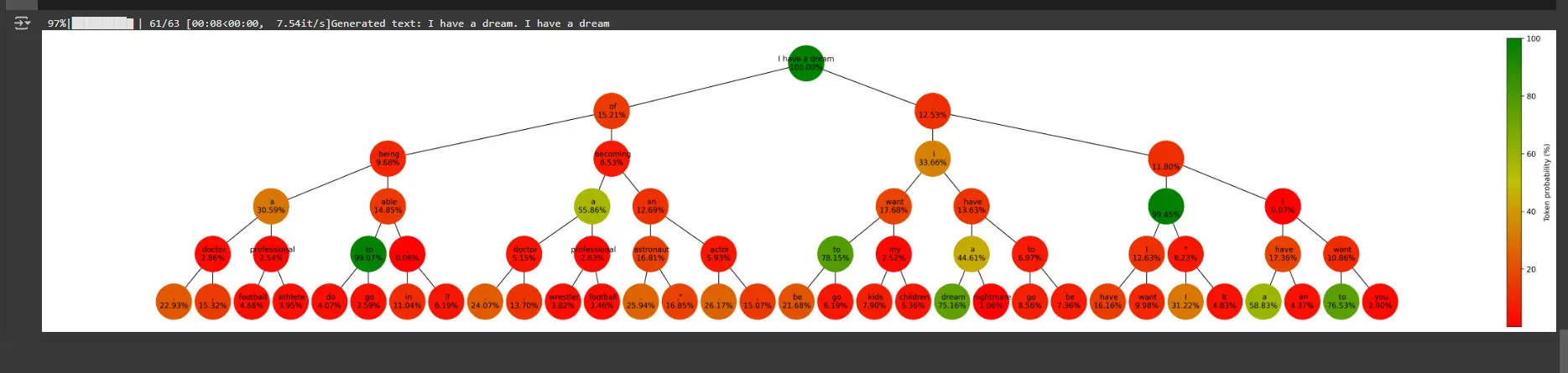
Step 7: Plot the Beam Search Graph

Visualizes the tree-like beam search graph.

def plot_graph(graph, size, beams, rating):
    fig, ax = plt.subplots(figsize=(3 + 1.2 * beams**size, max(5, 2 + size)), dpi=300, facecolor="white")

    # Create positions for every node
    pos = nx.nx_agraph.graphviz_layout(graph, prog="dot")

    # Normalize the colours alongside the vary of token scores
    scores = [data['tokenscore'] for _, information in graph.nodes(information=True) if information['token'] will not be None]
    vmin, vmax = min(scores), max(scores)
    norm = mcolors.Normalize(vmin=vmin, vmax=vmax)
    cmap = LinearSegmentedColormap.from_list('rg', ["r", "y", "g"], N=256)

    # Draw the nodes
    nx.draw_networkx_nodes(graph, pos, node_size=2000, node_shape="o", alpha=1, linewidths=4,
                           node_color=scores, cmap=cmap)

    # Draw the sides
    nx.draw_networkx_edges(graph, pos)

    # Draw the labels
    labels = {node: information['token'].break up('_')[0] + f"n{information['tokenscore']:.2f}%" 
              for node, information in graph.nodes(information=True) if information['token'] will not be None}
    nx.draw_networkx_labels(graph, pos, labels=labels, font_size=10)
    plt.field(False)

    # Add a colorbar
    sm = plt.cm.ScalarMappable(cmap=cmap, norm=norm)
    sm.set_array([])
    fig.colorbar(sm, ax=ax, orientation='vertical', pad=0, label="Token likelihood (%)")
    plt.present()

• Nodes signify tokens generated at every step, color-coded by their possibilities.
• Edges join nodes primarily based on how tokens prolong sequences.
• A colour bar represents the vary of token possibilities

Step 8: Primary Execution

# Parameters
size = 5
beams = 2

# Create a balanced tree graph
graph = nx.balanced_tree(beams, size, create_using=nx.DiGraph())
bar = tqdm(complete=len(graph.nodes))

# Initialize graph attributes
for node in graph.nodes:
    graph.nodes[node]['tokenscore'] = 100
    graph.nodes[node]['cumscore'] = 0
    graph.nodes[node]['sequencescore'] = 0
    graph.nodes[node]['token'] = textual content

# Carry out beam search
beam_search(input_ids, 0, bar, size, beams)

# Get the perfect sequence
sequence, max_score = get_best_sequence(graph)
print(f"Generated textual content: {sequence}")

# Plot the graph
plot_graph(graph, size, beams, 'token')

Rationalization

Parameters:

• size: Variety of tokens to generate (depth of the tree).
• beams: Variety of branches (beams) at every step.

Graph Initialization:

• Creates a balanced tree graph (every node has beams youngsters, depth=size).
• Initializes attributes for every node:(e.g., tokenscore, cumscore, token)
  • Beam Search: Begins the beam search from the foundation node (0)
  • Greatest Sequence: Extracts the highest-scoring sequence from the graph
  • Graph Plot: Visualizes the beam search course of as a tree.

Output:

You’ll be able to entry colab pocket book right here

Challenges in Beam Search

Regardless of its benefits, beam search has some limitations:

• Beam Measurement Commerce-off
• Repetitive Sequences
• Bias Towards Shorter Sequences

Regardless of its benefits, beam search has some limitations:

• Beam Measurement Commerce-off: Choosing the proper beam width is difficult. A small beam dimension would possibly miss the perfect sequence, whereas a big beam dimension will increase computational complexity.
• Repetitive Sequences: With out further constraints, beam search can produce repetitive or nonsensical sequences.
• Bias towards Shorter Sequences: The algorithm would possibly favor shorter sequences due to the best way possibilities are collected.

Conclusion

Beam search is a cornerstone of recent NLP and sequence era. By sustaining a steadiness between exploration and computational effectivity, it allows high-quality decoding in duties starting from machine translation to inventive textual content era. Regardless of its challenges, beam search stays a most popular selection resulting from its flexibility and skill to supply coherent and significant outputs.

Understanding and implementing beam search equips you with a robust instrument to reinforce your NLP fashions and purposes. Whether or not you’re engaged on language fashions, chatbots, or translation programs, mastering beam search will considerably elevate the efficiency of your options.

Key Takeaways

• Beam search is a decoding algorithm that balances effectivity and high quality in sequence era duties.
• The selection of beam width is vital; bigger beam widths enhance high quality however enhance computational value.
• Variants like various and constrained beam search enable customization for particular use circumstances.
• Combining beam search with sampling methods enhances its flexibility and effectiveness.
• Regardless of challenges like bias towards shorter sequences, beam search stays a cornerstone in NLP.

Regularly Requested Questions

The media proven on this article will not be owned by Analytics Vidhya and is used on the Writer’s discretion.

I am Neha Dwivedi, a Information Science fanatic , Graduated from MIT World Peace College,Pune. I am enthusiastic about Information Science and rising developments with it. I am excited to share insights and study from this group!